Click here to go see the bonus panel!
Hovertext:
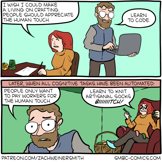
The alternative was artisanal soap biiiiiitch.
Today's News:
Hovertext:
The alternative was artisanal soap biiiiiitch.


Employees who are impressed by vague corporate-speak like “synergistic leadership,” or “growth-hacking paradigms” may struggle with practical decision-making, a new Cornell study reveals.
Published in the journal Personality and Individual Differences, research by cognitive psychologist Shane Littrell introduces the Corporate Bullshit Receptivity Scale (CBSR), a tool designed to measure susceptibility to impressive-but-empty organizational rhetoric.
“Corporate bullshit is a specific style of communication that uses confusing, abstract buzzwords in a functionally misleading way,” said Littrell, a postdoctoral researcher in the College of Arts and Sciences. “Unlike technical jargon, which can sometimes make office communication a little easier, corporate bullshit confuses rather than clarifies. It may sound impressive, but it is semantically empty.”
Although people anywhere can BS each other – that is, share dubious information that’s misleadingly impressive or engaging – the workplace not only rewards but structurally protects it, Littrell said. In a work setting where corporate jargon is already the norm, it’s easy for ambitious employees to use corporate BS to appear more competent or accomplished, accelerating their climb up the corporate ladder of workplace influence.
Corporate BS seems to be ubiquitous – but Littrell wondered if it is actually harmful. To test this, he created a “corporate bullshit generator” that churns out meaningless but impressive-sounding sentences like, "We will actualize a renewed level of cradle-to-grave credentialing” and “By getting our friends in the tent with our best practices, we will pressure-test a renewed level of adaptive coherence.”
He then asked more than 1,000 office workers to rate the “business savvy” of these computer-generated BS statements alongside real quotes from Fortune 500 leaders. Divided into four distinct studies, the research verified the scale as a statistically reliable measure of individual differences in receptivity to corporate bullshit, then, through use of established cognitive tests, made connections between receptivity to BS and analytic thinking skills known to be essential to workplace performance.
The results revealed a troubling paradox. Workers who were more susceptible to corporate BS rated their supervisors as more charismatic and “visionary,” but also displayed lower scores on a portion of the study that tested analytic thinking, cognitive reflection and fluid intelligence. Those more receptive to corporate BS also scored significantly worse on a test of effective workplace decision-making.
The study found that being more receptive to corporate bullshit was also positively linked to job satisfaction and feeling inspired by company mission statements. Moreover, those who were more likely to fall for corporate BS were also more likely to spread it.
Essentially, the employees most excited and inspired by “visionary” corporate jargon may be the least equipped to make effective, practical business decisions for their companies.
“This creates a concerning cycle,” Littrell said. “Employees who are more likely to fall for corporate bullshit may help elevate the types of dysfunctional leaders who are more likely to use it, creating a sort of negative feedback loop. Rather than a ‘rising tide lifting all boats,’ a higher level of corporate BS in an organization acts more like a clogged toilet of inefficiency.”
When BS goes too far or gets called out, real reputational or financial damage can occur, Littrell said. For instance, a leaked 2009 Pepsi marketing presentation with language such as “The Pepsi DNA finds its origin in the dynamic of perimeter oscillations…our proposition is the establishment of a gravitational pull to shift from a transactional experience to an invitational expression …” led to widespread ridicule in various news outlets.
And in 2014, a memo from the former executive vice president of Microsoft Devices Group to employees, later dubbed in the press “the worst email ever,” opened with 10 paragraphs of jargon, including “Our device strategy must reflect Microsoft’s strategy and must be accomplished within an appropriate financial envelope,” burying the real news in paragraph 11 – that 12,500 employees were going to lose their jobs.
Overall, the findings suggest that while “synergizing cross-collateralization” might sound impressive in a boardroom, this functionally misleading language can create an informational blindfold in corporate cultures that can expose companies to reputational and financial harm.
Littrell’s scale offers practical applications and could someday provide insights into job candidates' analytic thinking and decision-making tendencies. More work needs to be done, but for now, it’s a promising tool for researchers, Littrell said.
Researching BS also points out the importance of critical thinking for everyone, inside the workplace and out.
“Most of us, in the right situation, can get taken in by language that sounds sophisticated but isn’t,” Littrell said. “That’s why, whether you’re an employee or a consumer, it’s worth slowing down when you run into organizational messaging of any kind – leaders’ statements, public reports, ads – and ask yourself, ‘What, exactly, is the claim? Does it actually make sense?’ Because when a message leans heavily on buzzwords and jargon, it’s often a red flag that you’re being steered by rhetoric instead of reality.”
An open-access version of the study is available here.
Kate Blackwood is a writer for the College of Arts and Sciences.

AsteroidOS 2.0 runs Linux natively on smartwatches. Here's how to port your React app to a 1.4-inch screen.
Continue reading JavaScript on Your Wrist: Porting React/Vue Apps to AsteroidOS 2.0 on SitePoint.
A Denver company that developed legal software tried. They failed.
A game studio that made software for Disney tried. They spent over a year and hundreds of thousands of dollars. They had a team of programmers in Armenia, overseen by an American PhD in mathematics. They failed.
Commodore Computers tried. After three months of staring at the source code, they gave up and mailed it back.
Steam looked at it once, during the Greenlight era. "Too niche," they said. "Nobody will buy it. And if they do, they'll return it."
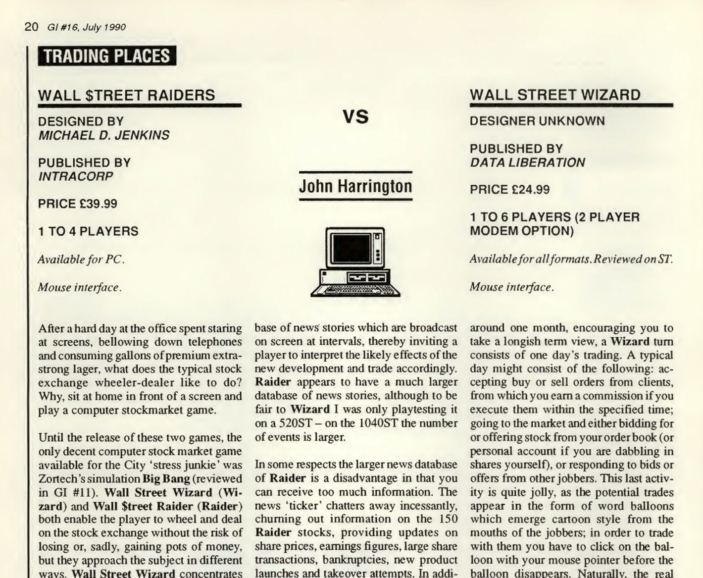
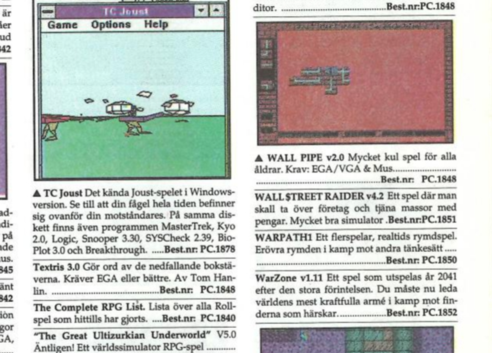
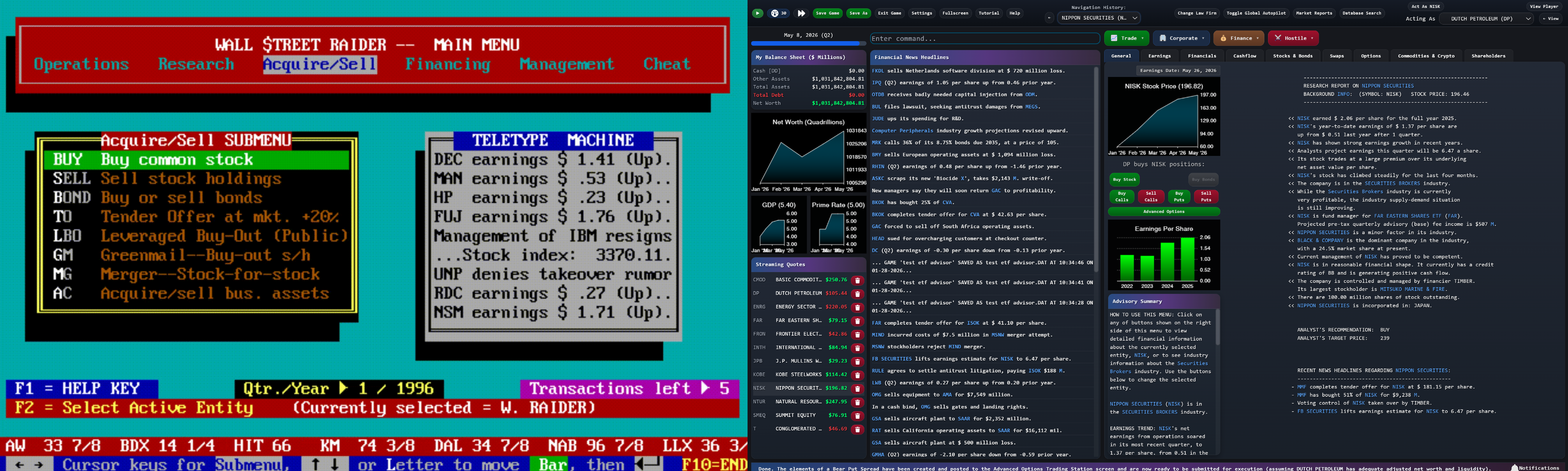
For nearly four decades, Wall Street Raider existed as a kind of impossible object—a game so complex that its own creator barely understood parts of it, written in a programming language so primitive that professional developers couldn't decode it. The code was, in the creator's own words, "indecipherable to anyone but me."
And then, in January 2024, a 29-year-old software developer from Ohio named Ben Ward sent an email.
Michael Jenkins, 80 years old and understandably cautious after decades of failed attempts by others, was honest with him: I appreciate the enthusiasm, but I've been through this before. Others have tried—talented people with big budgets—and none of them could crack it. I'll send you the source code, but I want to be upfront: I'm not expecting miracles.
A year later, that same 29-year-old would announce on Reddit: "I am the chosen one, and the game is being remade. No ifs, ands, or buts about it."
He was joking about the "chosen one" part. Sort of.
This is the story of how Wall Street Raider—the most comprehensive financial simulator ever made—was born, nearly died, and was resurrected. It's a story about obsession, about code that takes on a life of its own, about a game that accidentally changed the careers of hundreds of people. And it's about the 50-year age gap between two developers who, despite meeting in person for the first time only via video call, would trust each other with four decades of work.
Harvard Law School, 1967
Michael Jenkins was supposed to be studying. Instead, he was filling notebooks with ideas for a board game.
Not just any board game. Jenkins wanted to build something like Monopoly, but instead of hotels and railroads, you'd buy and sell corporations. You'd issue stock. You'd execute mergers. You'd structure leveraged buyouts. The game would simulate the entire machinery of American capitalism, from hostile takeovers to tax accounting.
There was just one problem: it was impossible.
"Nobody's going to have the patience to do this," Jenkins realized as he stared at his prototype—a board covered in tiny paper stock certificates, a calculator for working out the math, sessions that stretched for hours without reaching any satisfying conclusion.
The game he wanted to make required something that didn't exist yet: a personal computer.
So Jenkins waited. He graduated from Harvard Law in 1969. He worked as an economist at a national consulting firm. He became a CPA at one of the world's largest accounting firms. He practiced tax law at a prestigious San Francisco firm, structuring billion-dollar mergers—the exact kind of transactions he dreamed of simulating in his game.
And all the while, he kept filling notebooks.

1983
Sixteen years after those first notebooks, Jenkins finally got his hands on what he'd been waiting for: a Kaypro personal computer.
It had a screen about five inches across. It ran CP/M, an operating system that would soon be forgotten when MS-DOS arrived. It was primitive beyond belief by modern standards.
It was perfect.
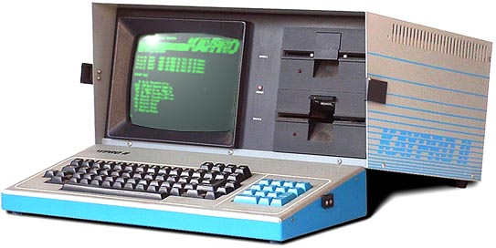
Jenkins pulled out a slim booklet that came with the machine—a guide to Microsoft Basic written by Bill Gates himself. He'd never written a line of code in his life. He had no formal training in computers. But that night, he sat down and typed:
10 PRINT "HELLO"
20 END
The computer said hello.
"As soon as I did that," Jenkins later recalled, "I realized: oh, this isn't that complicated."
What happened next became the stuff of legend in the small community of Wall Street Raider devotees. Jenkins stayed up until five in the morning, writing "all kinds of crazy stuff"—fake conversations that would prank his friends when they sat down at his computer, little programs that seemed to know things about his visitors.
It was a hoot. It was also the beginning of an obsession that would consume the next four decades of his life.
Within a year, Jenkins had built something he actually wanted: the first crude version of Wall Street Raider. It already had a moving stock ticker scrolling across that tiny five-inch screen. It already had news headlines streaming past. It was ugly and incomplete, but it was real.
Meanwhile, his law practice was suffering. "I was sitting in my office programming instead of drumming up business," he admitted. Only his side business—a series of tax guides called "Starting and Operating a Business" that would eventually sell over a million copies across all fifty states—kept him financially afloat.
The Late 1980s, 3:00 AM
The most complex parts of Wall Street Raider weren't written during normal working hours. They were written in the dead of night, in what Jenkins called "fits of rationality."
Picture this: It's three in the morning. Jenkins is hunched over his computer, trying to work out how to code a merger. Not just any merger—a merger where every party has to be dealt with correctly. Bondholders. Stockholders. Option holders. Futures positions. Interest rate swap counterparties. Proper ratios for every facet. Tax implications for every transaction.
"I felt like if I go to bed and I get up in the morning, I won't remember how to do this. So I just stayed up until I wrote that code."
— Michael Jenkins
The result? Code that worked perfectly—code that he tested for years and knew was correct—but code that even he didn't fully understand anymore.
"When I look at that code today, I still don't really quite understand it," he admitted. "But I don't want to mess with it."
This became the pattern. Jenkins would obsess over a feature until the logic crystallized in his mind, usually sometime after midnight, and then race to get it coded before the fragile understanding slipped away. The game grew layer by layer, each new feature building on the ones before, each line of code a record of what Jenkins understood about corporate finance at that particular moment in his life.
Years later, Ben Ward would give this phenomenon a name: The Jenkins Market Hypothesis.
"The hypothesis," Ward wrote in an email to Jenkins, "is that asset prices in the game reflect competition between Michael Jenkins' understanding of how Wall Street Raider worked at the point in time that he wrote the code over the past 40 years."
In other words: the game's simulated market was really just forty different versions of Michael Jenkins, from forty different stages of his life, all competing with each other.
Jenkins loved the theory. "I think it's very much related to chaos theory," he replied.
1986–2020
In 1986, Michael Jenkins retired from law and CPA practice at the age of 42. His tax guides were selling well, and his publisher had agreed to release Wall Street Raider. He thought he might spend a few years polishing his hobby project.
Thirty-four years later, he was still at it.
"I chuckle when I get emails from customers who ask me when the team is going to do one thing or the other. Well, the team is me. Ronin Software is definitely a one horse operation and always has been."
— Michael Jenkins
The game that started as a Monopoly variant had become something monstrous and magnificent. By the time Jenkins was done, Wall Street Raider contained:
Hidden beneath all this machinery was something that didn't dawn on most players until they'd been immersed in the game for months or years: an enormous amount of text. New events, scenarios, and messages would continue to pop up long after a player thought they'd seen everything—often laced with Jenkins' trademark tongue-in-cheek graveyard humor. The game wasn't just deep mechanically; it was deep narratively, in ways that only revealed themselves over time.
The game had, in short, become the most comprehensive financial simulator ever created—so complex that most people bounced off it, but those who broke through became devoted for life.
"The Dwarf Fortress of the stock market."
— what players call Wall Street Raider
Jenkins played chess against the world. He'd release a new feature, and within weeks, some clever player would email him: "Man, I found how to make trillions of dollars overnight with that new feature."
"I felt at times like the IRS plugging loopholes," Jenkins admitted. Every exploit became a patch. Every patch created new edge cases. The code grew more intricate, more layered, more incomprehensible to anyone but its creator.
And then something strange started happening.
Circa 2015
The emails started arriving from around the world, and they weren't about bugs.
One came from the Philippines:
"I've been playing your game since I was 13 years old, living in a third world country. Couldn't even afford to buy the full version. So I played the two-year demo for years and years. And it taught me so much that now I'm working for Morgan Stanley as a forex trader in Shanghai."
Another came from a hedge fund manager:
"I played Wall Street Raider for years and noticed that buying cheap companies—companies with low PE ratios—and turning them around seemed very profitable in the game. But I wasn't doing that with my real clients. I wasn't doing well. Finally I decided to just start doing what I'd been doing in Wall Street Raider."
He attached a document: an audited report from Price Waterhouse, showing a 10-year period where he'd averaged a 44% compounded annual return using strategies he'd learned from a video game.
"Your game has changed my life."
Jenkins heard it again and again. From CEOs. From investment bankers. From traders and professors and finance students. People who'd played the free demo version as teenagers in developing countries and parlayed what they learned into careers at Goldman Sachs and Morgan Stanley. People who'd been stone masons wondering if they could do something more.
By his own count, over 200 CEOs and investment bankers had reached out over the years to say that Wall Street Raider had shaped their careers.
"I created the game because it was fun to do so," Jenkins said. "But I've been pleasantly surprised to see the positive impact it has had on the lives of a lot of people who grew up playing it for years and years."

It was, it turned out, not just a game. It was accidentally one of the most effective financial education tools ever created—a simulator so realistic that its lessons transferred directly to real markets.
Various Years
Everyone wanted to modernize Wall Street Raider. Everyone failed.
The interest was obvious. Here was a game with proven educational value, devoted fans, and gameplay depth that put most competitors to shame. The only problem was the interface—a relic of the 1990s Windows era, all dropdown menus and tiny text boxes and graphics that looked, as one longtime player put it, "like they came from the dark ages."
So they came, the would-be saviors, with their teams and their budgets and their ambitions.
A Denver company that developed legal software sent their programmers. They couldn't make it work.
A game studio that did work for Disney assembled a team in Armenia, overseen by an American PhD in mathematics. They spent over a year and "lots of money"—by some accounts, hundreds of thousands of dollars—trying to port the game to iPad.
"None of their people had the kind of in-depth knowledge of corporate finance, economics, law, and taxation that I was able to build into the game," Jenkins explained. "So they simply couldn't code the simulation correctly when they didn't have a clue how it should work."
They gave up.
Commodore Computers, back in 1990, licensed the DOS version. After three months of trying to understand the source code, they mailed it back.
Steam, during the Greenlight era, rejected it outright. "Too niche," they said. "Almost no graphics. Looks clumsy and primitive."
The pattern was always the same. Professional programmers would look at Jenkins' 115,000 lines of primitive BASIC—code that "broke all the rules for good structured programming"—and try to rewrite it in something modern. C++, usually. They'd make progress for a while, get 60% or 80% of the way there, and then hit a wall.
The problem wasn't technical skill. The problem was that to rewrite the code, you had to understand the code. And to understand the code, you had to understand corporate finance, tax law, economics, and securities regulation at the same depth as someone who'd spent decades as a CPA, tax attorney, and economist.
Those people didn't tend to become video game programmers.
"My 115,000 lines of primitive BASIC source code," Jenkins admitted, "was apparently indecipherable to anyone but me."
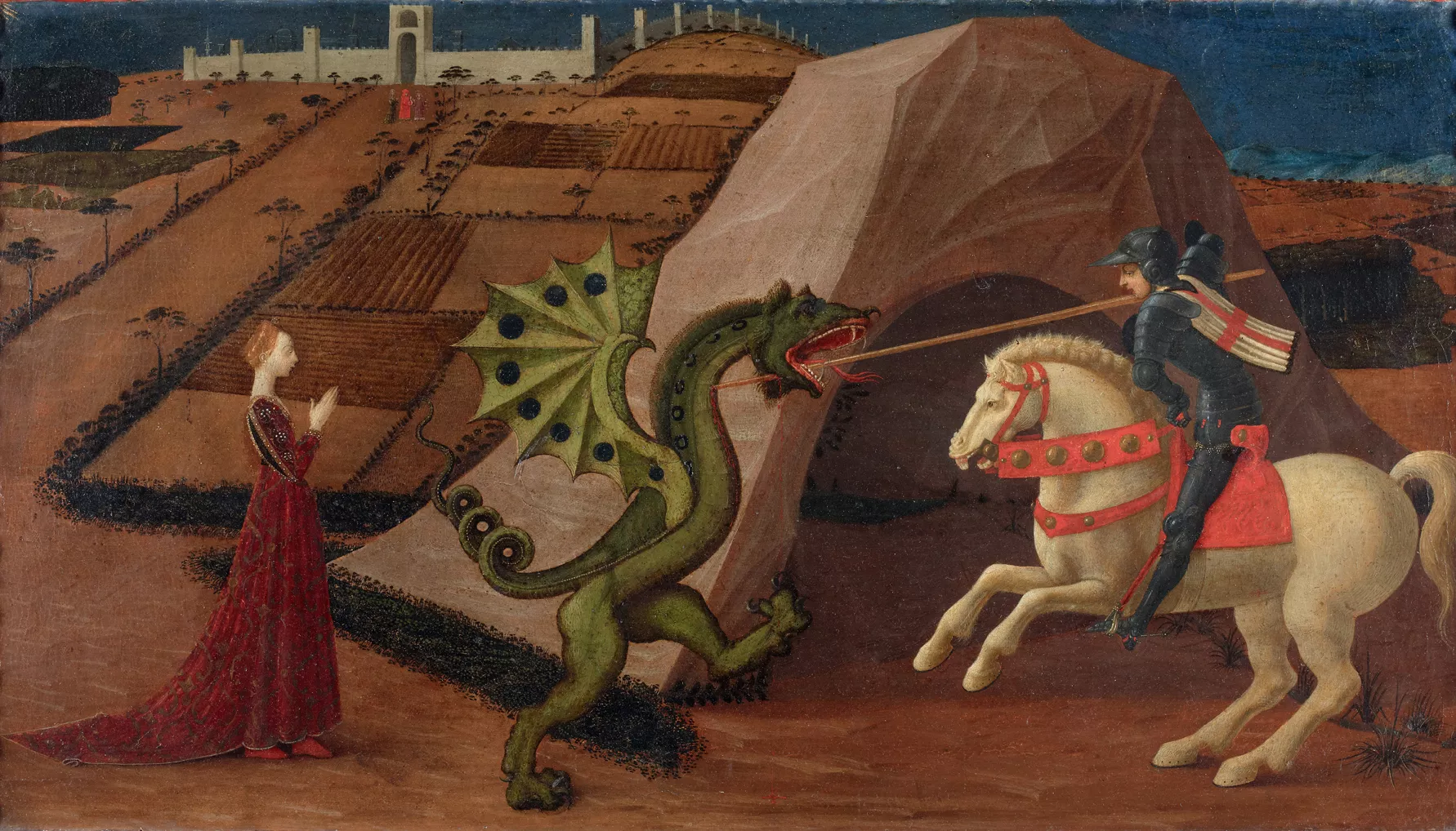
The skeletons piled up around the dragon.
2020–2023
By his late seventies, Michael Jenkins was running out of options.

His e-commerce provider had gone bankrupt, taking six months of income with them. Payment processors kept rejecting him—some because of obscure tax complications from selling software in hundreds of countries, others because their legal departments didn't want to be associated with anything finance-related. For a period, you literally couldn't buy Wall Street Raider anywhere.
"At one point the challenges got so overwhelming," Jenkins admitted, "that I seriously considered just shutting down everything."
In 2020, a gaming journalist named AJ Churchill sent Jenkins a simple email asking whether upgrades to Speculator (a companion game) were included in the purchase price.
Jenkins' response was... more than Churchill expected:
"Also, as a registered user, you can buy Wall Street Raider at the discounted price of $12.95. As I make revisions over a period of a year or two, I eventually decide when I've done enough that it's time to issue an upgrade version, but there is no timetable. And to be frank, I'm running out of feasible ideas for improvements to both games, and there may only be one or two more upgrades to either program.
Otherwise, at age 76, I may be finally coming near the end of development with my limited software skills, unless I can license my code to a large software/game company that is willing to hire the kind of expensive programming talent that writes software for firms like Merrill Lynch or Goldman Sachs—who would be the only programmers capable of porting my game to iOS, Android, or to a classy-looking Windows GUI. And that is very unlikely.
I've pretty much given up on the idea of anyone ever being able to port it."
Churchill posted the exchange to the r/tycoon subreddit with the title: "I reached out to the 79-year-old creator of Wall Street Raider and here's what he wrote back."
The post got some attention. People commented about what a shame it was. A few bought the game out of curiosity. And then, like most Reddit posts, it faded into obscurity.
Hear the story from Michael Jenkins and Ben Ward themselves.
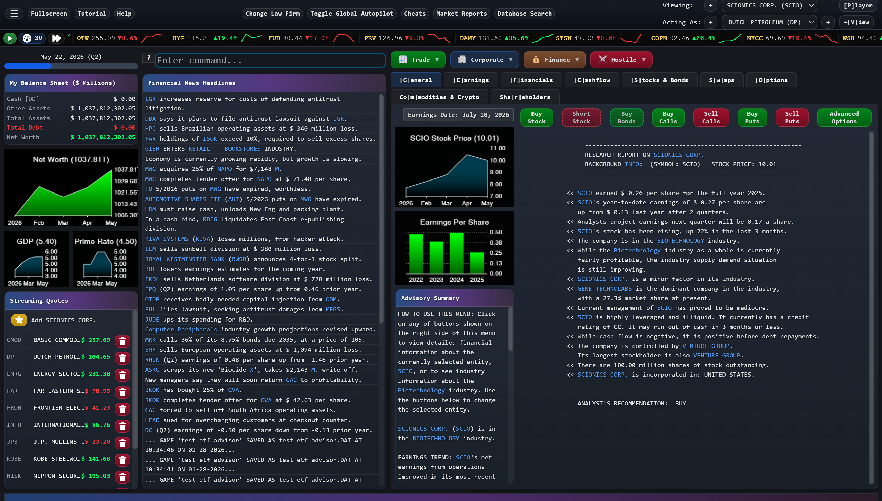
But somewhere in Ohio, a young software developer read it. And he couldn't get the image of a Bloomberg terminal out of his head.
Meanwhile, in Ohio
Ben Ward's first memory of programming was going to the library as a small child and checking out a massive textbook on C++ game development.
"I barely probably knew how to read at that point," he recalled. "I had no idea how to install a compiler, run the code that was in this book. But it just kind of got me thinking."
Ward was, by his own admission, a terrible student. He had ADHD that went undiagnosed until adulthood. He spent more time helping his classmates with their homework than doing his own. His two-year programming degree took five years to complete.

But when it came to code, something clicked.
At 18, working at his uncle's manufacturing company, Ward built a management system in three months that replaced their spreadsheets. It ran the business for five years. He went on to build ERP and warehouse management systems, worked at fintech companies, and became a senior full-stack developer.
And then, just for fun, he took on a challenge: porting Colossal Cave Adventure—the legendary 1976 text adventure game—from its original Fortran code to Lua, so it could run on the Pico-8 fantasy console.
The Fortran manual was a thousand pages. Ward had never written Fortran in his life. He wrote a transpiler—a program that converts one programming language to another—and had Colossal Cave running on Pico-8 in eight hours.
"If it wasn't for that project," Ward later said, "I don't think I would have had the confidence to do this. Because of course, this was about a thousand times harder."
January 2024
Ben Ward found AJ Churchill's Reddit post while looking for stock market games to use as inspiration. He was thinking about making his own financial simulator, something with the depth he couldn't find anywhere else.
Then he discovered that the depth already existed. It just looked like it was from 1995.
Ward paid $30 for Wall Street Raider. He lost terribly for several hours. He bought the $20 manual and read all 271 pages. He was still terrible at the game.
"That's when I realized," Ward said. "This game has amazing depth. Even knowing all the rules, even memorizing all the opening moves, you still need to practice. It's like chess."
He couldn't get the image of Wall Street Raider with a Bloomberg terminal interface out of his head.
So he emailed Michael Jenkins.
Jenkins had been through this before. Over the years, developers had reached out wanting to modernize the game—promising modern graphics, mobile ports, the works. Every one of them had eventually given up. He was candid with Ward about the history:
I appreciate what you're saying, but I have to be honest—I've heard this before. A Denver legal software company tried. A Disney game studio tried. Teams of people spent hundreds of thousands of dollars and years of effort. None of them could pull it off. I'd love to be wrong, but I've learned not to get my hopes up.
Ward was persistent. Months of emails followed. Long, detailed messages about his vision, his technical approach, his background. Jenkins, cautiously optimistic, decided to give him a chance.
"Here's the source code. Let's see what you can do."
Jenkins made Ward sign an NDA—snail-mailed, because Jenkins was old school. Ward signed it, mailed it back, and received the 115,000 lines of BASIC code that represented forty years of work.
After that, the communications between them tapered off. Jenkins went back to his own work. Ward went quiet.
2024
For twelve months, Ben Ward did almost nothing but read.
He read the 2,000-page Power Basic manual. (Power Basic was the language Jenkins used—a company that was now defunct, its compiler preserved on GitHub among other places.) He re-read Wall Street Raider's 300-page game manual. He read through years of Power Basic forum posts.
"Over the course of that year," Ward estimated, "I probably spent 90% of the time reading. I wasn't really coding at all."
The feeling of failure visited him often: I'm going to be like everybody else. I can't do it. I'm not smart enough.
But Ward kept coming back to one question: Why did everyone else fail?
The Denver developers had failed. The Disney team had failed. Commodore had failed. Hundreds of thousands of dollars, gone.
"And I realized it's because they keep trying to rewrite the code," Ward said. "They keep trying to convert Power Basic to C++ or some other language, and it doesn't work."
"Don't rewrite. Layer on top."
— Ben Ward's breakthrough insight
The insight was elegant: instead of rewriting Jenkins' code, wrap a modern interface around it—the same approach enterprise companies use to modernize legacy systems every day. Keep the engine. Replace the dashboard.
After months of experimentation, Ward found a way to bridge modern code to Jenkins' untouched Power Basic engine. He tried it one day. A simple button. Some text.
It worked.
Late 2024
Ward sent Jenkins a message: a screen recording of his prototype. A button. Some text. Nothing fancy.
"This isn't anything," Ward wrote. "But this is it. Now I can use my skills to layer on top of the old engine."
Jenkins was astonished.
"When I finally reached out to Ben recently to see how he was doing, I was astonished to learn that he had spent the past year studying my code. Unlike all the other people who had tried and failed, he'd not only figured out how to overlay a new user interface onto the old framework of game logic—he'd also reworked many of the screens and just generally made the thing a lot better."
That was when everything changed.
Jenkins asked what he could do to help. Ward mentioned that the biggest bottleneck was the cryptic variable names—short abbreviations that were common in old-school programming but made the code nearly impossible to follow.
Three days later, Jenkins sent back the entire codebase with every variable renamed.
"He not only commented everything," Ward marveled, "he went through every single line of code and renamed every single variable for me in about three days. Using search and replace, because there's no IDE rename feature. And he did it flawlessly—no bugs, no side effects."
In total, Michael Jenkins and Ben Ward had two phone calls. One video call. Everything else was email.
"This guy entrusted me with 40 years of his Opus Magnum," Ward said, "all based on email."
2025
The first time Ward streamed the working game on Discord, thirty people showed up immediately.
He played his opening strategy—finding a company being sued and buying calls on the plaintiff—and made ten or twenty billion dollars in twenty minutes.
"And then I kind of just sat back," Ward recalled, "and I was like: Oh my god. It works. And it's fun."
Two years of work. Reading. Debugging. Doubting himself. And now it was real.
The Steam page went live. The open beta began. Bug reports flooded in—mostly for Ward's new code, almost never for Jenkins' battle-tested engine. Ward had done a "hostile takeover" of the dead subreddit (via Reddit's request process) and grown it from 200 users to thousands. A Discord server filled with strategy discussions and feature requests and players who'd been waiting years for this moment.
Ward, joking but not joking, posted on Reddit: "I am the chosen one, and the game is being remade."
"I mean, I was joking about 'the chosen one,'" he admitted later. But AJ Churchill, the journalist whose Reddit post had started everything, pushed back:
"Your life has led you to this moment. You worked in finance. You worked as a developer. You literally translated a game from the 1970s onto another platform. You were lab-grown to be the perfect person to work on this."
Jenkins, for his part, had found something he'd given up hoping for: someone to pass the torch to.
"I'm basically passing the Wall Street Raider torch on to Ben," Jenkins announced in a video to the community. "And I hope that its impact will endure for many more years, long after I'm gone."

Then he added a warning:
"Just one word of warning. It will take over your life."
Ward's response: "It already has. I can't escape from it now."
Michael Jenkins is 81 years old.
Will Crowther, creator of Colossal Cave Adventure—the same game Ben Ward ported to Pico-8—is 89.
"I guess that technically makes me the second oldest," Jenkins observed.
He jokes about mortality. "I plan to live forever," he says. "However, that's not too likely, I'm told."
The Wall Street Raider community jokes about it too. When Ward mentioned that release would happen "barring I don't get hit by a bus," the Discord erupted: "All bus schedules in Ohio—we're turning them off. No more buses."
Ward has taken to assuring everyone: "I look both ways when I cross the street."
Behind the jokes is something serious: the knowledge that this is Jenkins' final effort to preserve what he built. "This will be my final effort to preserve my little piece of gaming history," he said.
But Ward has built something that will outlast both of them.
"One of the reasons I wanted to put it on Steam," Ward explained, "is that let's say a freak accident happens and Michael and I both get hit by a bus. Wall Street Raider will still live on, so long as Steam doesn't take the game down. It doesn't really depend on Michael and me anymore."
2025 and Beyond
From notebooks in a Harvard Law School dormitory in 1967 to a Steam store page in 2025: fifty-eight years.
The game that almost became abandonware is now being played by thousands. The code that was "indecipherable to anyone but me" is now being extended by a new generation. The financial education that accidentally changed hundreds of careers is reaching thousands more.
5,000+ Steam Wishlists
800 Discord Members
1,000+ Reddit Community
500+ Beta Testers
200+ Players with 100+ Hours
58 Years in the Making
The remaster isn't just a new coat of paint. Ward rebuilt the entire player experience around the way financial professionals actually work: a searchable help system built on Jenkins' 271-page strategy manual, a tutorial onboarding system that's continuously being refined, contextual tooltips that walk players through the game's most advanced mechanics, and hotkeys for every button, tab, and hyperlink—just like a real Bloomberg terminal—so experienced players can move at the speed of thought.
The game underneath is still Jenkins' 115,000 lines of battle-tested code. The interface on top is what it always deserved.
The comparison that keeps coming up is Dwarf Fortress. For years, it was the same story: legendary depth, a devoted niche community, held back by an interface that scared everyone else away. When it finally got a graphical overhaul and launched on Steam in 2022, it sold over 500,000 copies in two weeks. The parallel to Wall Street Raider is hard to miss.
And then there's the story itself. An 81-year-old Harvard Law grad who taught himself to code at midnight, passing four decades of work to a 30-year-old developer from Ohio who cracked the code that no one else could. That's not a marketing angle—it's a headline that writes itself.
Jenkins still can't fully stay away. When a longtime player known as Malor kept requesting cash flow statements for banks, Jenkins insisted it would be too hard and not very useful. Two days later, he emailed Ward: "So, I think I figured out how to do cash flow statements for banks, and I've been working on this code..." Malor's handle, incidentally, is a teleportation spell from The Bard's Tale—a 1985 RPG that was the first computer game he ever saw. Wall Street Raider was the first game he installed on every new PC he ever bought. After four decades of playing, he's now in the Discord server, helping to shape the remaster he'd waited a lifetime for.
"He acts like he doesn't know how the code works," Ward observed. "But he can't stop."
Neither can the players who've been waiting for this. Neither can the new players discovering for the first time that a game this deep exists.
Wall Street Raider is, finally, getting its Bloomberg terminal interface. But underneath, it's still the same game—115,000 lines of code written by forty different versions of Michael Jenkins, competing with each other across four decades, governed by what Ward calls "laws written on top of laws that were interpreted wrong."
It's grotesquely complex. Even the creator barely understands parts of it.
And it's alive.
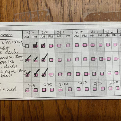
Recently I had to take my dog in for surgery. Over nearly 20 years of owning multiple dogs, this isn't new. But this is the first time design actually played a helpful role for my pet's post-op care.
At every other veterinary practice I've been to—over a half-dozen, from Manhattan to the rural countryside—they hand you med vials with the dosage instructions printed on them. The font on the labels is tiny (requiring reading glasses, for me) and it's impossible to read a full sentence without rotating the vial.

This time, however, this new vet handed me this simple chart:
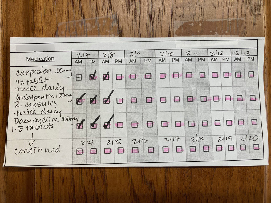
I was really impressed by the low-tech efficacy of the design. The days are delineated by tonal differences, and a pink highlighter was used on all but one of the boxes, to remind me that one of the drugs was not to be administered on the morning of 2/7 (due to lingering medication from the surgery, I was verbally told). Two of the drugs are meant to be administered for 7 days in a row, and the third for 14 days in a row; the vet tech was easily able to modify the chart to indicate this.
All of this information is on the three barely-legible labels on the vials. But by consolidating it into one chart, the vet practice made the information much easier to grasp and track.
I do wonder why, having been to so many vets, this is the first time I'd seen such a chart. It should be standard practice.